Matlab Program For Dolph Chebyshev Array Definition
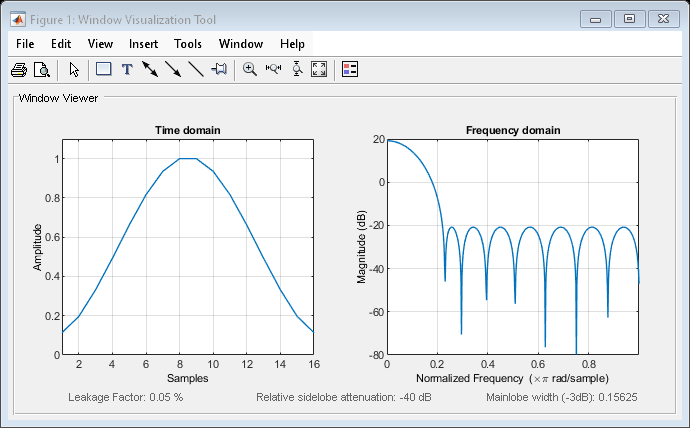
Algorithms An artifact of the equiripple design method used in chebwin is the presence of impulses at the endpoints of the time-domain response. This is due to the constant-level sidelobes in the frequency domain. The magnitude of the impulses are on the order of the size of the spectral sidelobes. If the sidelobes are large, the effect at the endpoints may be significant. For more information on this effect, see.
MATLAB Program for Chebyshev Array Antenna m file Dolph proposed (in 1946) a method to design arrays with any desired sidelobe levels and any HPBWs. This method is based on the approximation of the pattern of the array by a Chebyshev polynomial of order m, high enough to meet the requirement for the side- lobe levels. Antenna Arrays. It is tool to produce radiation pattern for following antenna arrays: 1. Binomial and 4. Dolph - Chebyshev Run.m file and enter the no. Of elements and distance to produce radiation pattern Optimization of codes has been done as a matter of practice. Suggestions are highly encouraged.
The equivalent noise bandwidth of a Chebyshev window does not grow monotonically with increasing sidelobe attenuation when the attenuation is smaller than about 45 dB. For spectral analysis, use larger sidelobe attenuation values, or, if you need to work with small attenuations, use a Kaiser window.
Antenna-Theory.com - Dolph-Chebyshef Weighting Example for Antenna Arrays Dolph-Chebyshev Example Previous: (Home) Page In the previous page on, the Dolph-Tschebysheff method was introduced. On this page, we'll run through an example. Consider a N=6 element array, with a sidelobe level to be 30 dB down from the main beam ( S=31.6223). We'll assume the array has half-wavelength spacing, and recall that the Dolph-Chebyshev method requires uniform spacing and the array to be steered towards broadside (and yes, everyone spells Chebyshef in a different way, which is why I keep changing the spelling). The array has an even number of elements, so we'll write the array factor as: Using the, the above equation can be rewritten as: We'll calculate our parameter ( ) as: Then we'll substitute for cos(u) into the last equation for the AF as described previously: We now have a polynomial of order N-1 = 5, so we'll use the Chebyshef polynomial T5(t), and equate that to our new array factor: The above equation is valid for all values of t. Hence, the terms that multiply t must equal, the terms that multiply t cubed must be equal, and the terms that multiply t to the 5th power must be equal. As a result, we have 3 equations and 3 unknowns, and we can easily solve for the weights: The resulting normalized AF is plotted in Figure 1.
Normalized array factor for the example on this page. Note that as desired, the sidelobes are equal in magnitude and 30 dB down from the peak of the main beam. The beamwidth obtained here (approximately 60 degrees) is the minimum possible beamwidth obtainable for the specified sidelobe level using any weighting scheme.
This is the Dolph-Tschebysheff method. The basic math is all used in designing digital filters that have equal-ripple filter characteristics in the pass and stop bands. Note that if you understand digital signal processing, weight selection in antenna arrays is simple. And if you've learned something about weighting methods in antenna arrays, you've learned something about designing filters for digital systems. The underlying mathematics is largely the same. Next: (Main) (Home) (Home). Sony vaio pcg 4121 drivers license.